I/O Parallelism
It is a form of parallelism in which the relations (tables) are partitioned on multiple disks a motive to reduce the retrieval time of relations from the disk. Within, the data inputted is partitioned and then processing is done in parallel with each partition. The results are merged after processing all the partitioned data. It is also known as data-partitioning.
Hash partitioning has the advantage that it provides an even distribution of data across the disks and it is also best suited for those point queries that are based on the partitioning attribute.
It is to be noted that partitioning is useful for the sequential scans of the entire table placed on ‘n‘ number of disks and the time taken to scan the relationship is approximately 1/n of the time required to scan the table on a single disk system. We have four types of partitioning in I/O parallelism:
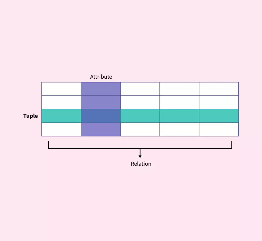
Figure 1: Tuple, Attribute, Relation
1. Hash partitioning
In hash partitioning, data is distributed across multiple disks based on a hash function applied to one or more partitioning attributes (such as a column in a table). This method ensures that data with the same attribute values is always sent to the same disk, making it ideal for quick lookups on specific values.
Here’s a detailed breakdown of how it works:
- Select Partitioning Attributes:
- Choose one or more attributes (e.g., a CustomerID or ProductID column) that will be used to determine the disk on which each tuple (row) will be stored.
- These attributes should ideally be chosen based on how data is queried. For example, if queries frequently involve customer lookups, CustomerID is a good choice.
- Apply a Hash Function:
- A hash function h is chosen with a defined range, typically from 0 to n-1, where n is the number of disks.
- The hash function takes the value(s) of the partitioning attribute(s) as input and outputs an integer (0, 1, 2, …, n-1 )
- Determine the Disk: Let i be the output from the hash function h. The resulting integer i corresponds to a specific disk where the tuple should be stored. For instance, if i=3, the tuple goes to Disk 3.
Example:
- Suppose we have 4 disks (Disk 0, Disk 1, Disk 2, and Disk 3), and we want to hash-partition a relation (table) based on the CustomerID attribute.
- We choose a hash function h(CustomerID) that maps CustomerID values into the range 0 to 3.
- For a row where CustomerID = 101, if h(101)=2, then this row would be stored on Disk 2.
Advantages:
- Efficient Point Queries: By hashing one or more attributes, this method can direct specific queries to only one disk based on the hash value. This allows point queries to access a single disk, keeping others free.
- Supports Indexing: Hash partitioning can work with indexing, which makes lookups and updates quicker and more efficient. Balanced Retrieval: A well-designed hash function distributes data evenly, ensuring balanced retrieval and reducing bottlenecks.
Limitations:
- Inefficient for Range Queries: Since hashing disperses data across disks based on hash values, related data isn’t clustered, making range queries difficult because they may require accessing multiple disks.
Best For: Point queries and sequential scans, where specific records or even distribution is essential.
Not Suitable For: Range queries, due to the scattering of related data across multiple disks.
2. Range partitioning
In range partitioning, data is divided across multiple disks based on specified value ranges of a partitioning attribute. This method groups tuples (rows) based on a defined partitioning vector, which contains boundary values, or "cut-off" points, to separate ranges. It is particularly useful for range-based queries, where you want to retrieve data that falls within certain intervals.
-
Select a Partitioning Attribute: Choose a single attribute (such as Age or Date) on which to base the partitioning. This attribute should be meaningful for range queries. For instance, partitioning by Date is useful for time-based queries.
-
Define a Partitioning Vector: Specify a list of boundary values, called a partitioning vector [𝑣0,𝑣1,…,𝑣𝑛−2], where each 𝑣𝑖 represents the start of a new range. For 𝑛 disks, you would have 𝑛 − 1 boundary values in this vector to create 𝑛 ranges.
-
Determine the Disk for Each Tuple:
- For each tuple (row), let 𝑣 be the value of the tuple in the partitioning attribute.
- Based on 𝑣 assign the tuple to a disk according to the following rules:
- Disk 0: If 𝑣 < 𝑣0 , the tuple goes to Disk 0.
- Disk 𝑖+1: If 𝑣𝑖 ≤ 𝑣 < 𝑣𝑖+1 , the tuple goes to Disk 𝑖+1.
- Disk 𝑛−1: If 𝑣 ≥ 𝑣 𝑛−2 , the tuple goes to the last disk (Disk 𝑛−1).
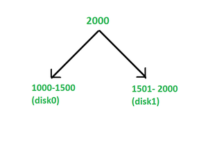
Example: Suppose we have 4 disks (Disk 0, Disk 1, Disk 2, Disk 3) and a partitioning vector [20,40,60]. If our partitioning attribute is Age, the data distribution would be:
- Disk 0: Ages below 20.
- Disk 1: Ages from 20 to below 40.
- Disk 2: Ages from 40 to below 60.
- Disk 3: Ages 60 and above.
Advantages:
- Data Clustering: Data is partitioned based on ranges of values within a specific attribute, meaning related data is stored together. This is beneficial for range queries where records within a range are accessed frequently.
- Efficient for Sequential and Point Queries: This method allows data to be located on specific disks based on the range, which makes it efficient for accessing ranges of records or specific records within that range.
- Less Disk Interference for Range Queries: Only disks containing relevant ranges are accessed, leaving other disks free for other operations.
Limitations:
Data Skew: If data distribution is uneven (many records fall within a few ranges), some disks may be overloaded, reducing the benefits of parallelism. Limited Parallelism: When data is highly concentrated in specific ranges, only a few disks are needed, reducing the system’s overall parallel efficiency.
Best For: Range and sequential access queries, where records within a range are accessed frequently.
Not Suitable For: Data distributions with heavy skew, as it can limit load balancing across disks.
3. Round-robin partitioning
In Round-robin partitioning, also referred to as "roulette" partitioning, data is distributed evenly across multiple disks (or nodes) by assigning each tuple (row) to a disk in a cyclical, rotating fashion.
Here’s how it works with the formula:
Assigning Data: For each row or tuple in the relation (table), assign it to a disk based on the formula:
disk = i mod n
where,
- 𝑖 = the position of the tuple in the sequence.
- n = the total number of disks available.
- i mod n = the remainder when 𝑖 is divided by 𝑛, determining which disk the tuple should be sent to.
Example: Suppose we have 4 disks (Disk 0, Disk 1, Disk 2, and Disk 3) and a relation with tuples in a sequence.
- T1 (first tuple) goes to Disk 1 % 4 = Disk 1.
- T2 (second tuple) goes to Disk 2 % 4 = Disk 2.
- T3 (third tuple) goes to Disk 3 % 4 = Disk 3.
- T4 (fourth tuple) goes to Disk 4 % 4 = Disk 0.
- T5 (fifth tuple) goes to Disk 5 % 4 = Disk 1.
This sequence repeats, cycling through the disks.
Advantages:
- Ideal for Sequential Scans: This technique distributes data evenly across all available disks by assigning each new tuple to the next disk in a round-robin fashion, ensuring that disks contain an almost equal number of tuples.
- Balanced Workload: Because all disks have a similar load, data retrieval is well-balanced across the system, which is especially useful for workloads that require reading large portions of data sequentially.
Limitations:
- Challenging for Point and Range Queries: Since data is scattered, retrieving specific subsets can require scanning multiple disks, making point and range queries more difficult and time-consuming.
- No Data Clustering: Data tuples are randomly distributed, so related data isn’t stored together on a single disk, impacting the efficiency of certain queries.
Best For: Sequential scans, where the goal is to read large portions of data.
Not Suitable For: Point queries (queries targeting specific records) and range queries, as these require accessing multiple disks.
4. Schema partitioning
In schema partitioning, different tables within a database are placed on different disks. See figure 2 below:

Advantages:
Simplicity in Management: Data is organized based on the schema structure, making it easier to locate and manage as per the database design. Data Locality: Related data within the same schema can be stored together, improving access times for schema-bound queries.
Limitations:
- Limited Flexibility: Schema-based organization restricts the data layout, making it challenging to adapt if the data access patterns change or are diverse.
- Imbalanced Load: Different schema sizes or data amounts can create an uneven distribution, with some disks potentially more loaded than others.
Best For: Workloads heavily organized by schema, where queries often target data within the same schema.
Not Suitable For: Workloads with dynamic or highly varied queries, as these might require more flexible partitioning.
Comparison of Partitioning Techniques
| Partitioning Technique | Advantages | Limitations | Best For | Not Suitable For |
|---|---|---|---|---|
| Round-Robin | - Best suited for sequential scans - Balanced retrieval work across disks | - Difficult for point and range queries - No clustering as tuples are scattered across disks | Sequential scans | Point and range queries |
| Hash Partitioning | - Efficient for point queries by accessing a single disk - Can support indexing for fast lookup and updates - Balanced retrieval with good hash function | - No clustering, making range queries challenging | Point queries and sequential scans | Range queries |
| Range Partitioning | - Allows for data clustering based on partition attribute - Efficient for sequential access and point queries - Limited disks accessed for range queries, leaving others free | - Data skew can reduce parallelism if tuples are concentrated on a few disks - Not suitable if tuples aren’t distributed across blocks | Sequential access, range queries, and point queries | Scenarios with data skew |
| Schema Partitioning | - Simplifies management with schema-based allocation - Data locality based on schema organization | - Limited flexibility for dynamic or varied queries - Less balanced workload if schemas differ in size | Schema-organized workloads | Dynamic or highly varied queries |